A note about Measuring the G2G response times which includes overshoot

One note that we mentioned earlier about the “Complete Response Time” (0 – 100%) is that it will incorporate the overshoot time as well. It measures the full time it takes to go from the starting grey shade, to the final grey shade AFTER any overshoot has taken place. It’s the time it takes to reach and settle on the grey shade it was trying to reach, not when it first reaches that shade before the overshoot appears. This basically captures the length of the overshoot in the response time figure as well.

For the “Complete Response Time” on the graph it would be measuring the time between the two yellow lines for example: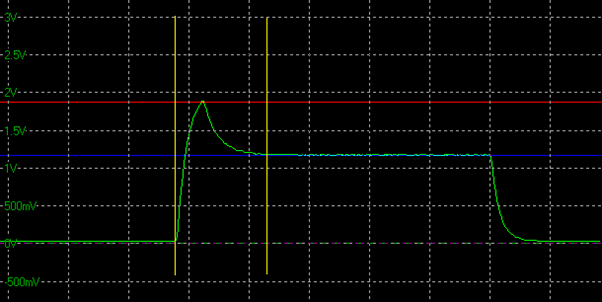

Initial Response Time vs. Perceived Response Time

In the calculation you will see two response times presented in your data – regardless of which other settings you have choosen. These are the “initial response time” and the “perceived response time”. These will both consider any overshoot differently.

Initial Response Time

This is the method that has been used in the market for a long time. The response time is measured on the part of the curve BEFORE the overshoot peak. It captures how long it takes to reach the desired shade, or to the desired tolerance level, but ignores the fact that the screen then overshoots this shade and then takes a while to reach back down. It would be capturing the time between the two yellow lines on the below graph: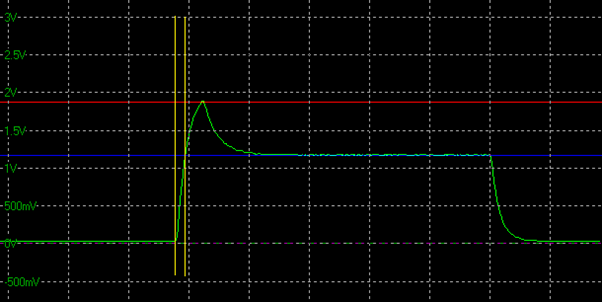

The problem with this is that it does not then capture in that response time figure the fact that there is an overshoot, and in reality it will take quite a bit longer to reach back to the desired end grey shade. Is it fair to reward a screen with a very low response time G2G figure when the overshoot might take a long time to disappear?

In this “initial response time” approach the overshoot is not forgotten, it is represented in a separate table showing the severity of the overshoot peak, preferably using gamma corrected RGB overshoot as discussed above.

It is still fine to present the “initial response time” in this way, but if overshoot is present this must be considered and presented alongside the G2G response times. This is the approach that has been used in the market for 20+ years so is the most widely recognised, and easiest to provide comparisons with over all the years’ worth of testing.

Pereceived Response Time

This is an alternative approach and is presented in the output data of any measurement. If overshoot is present it is captured in the G2G response time figure as well, representing the time it takes to settle back down to the final shade (or close to it when using a tolerance level) AFTER any overshoot has disappeared. It is the “perceived response time” as it considers the impact of the overshoot in the G2G figures. This may be a useful method to use if you wanted to show fewer data sets in your results, or were not including a normal overshoot table for instance.

On the graph it would look like this: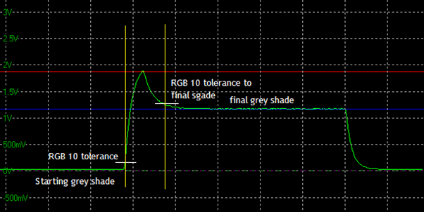

So keep in mind that if you are presenting the “complete response time” or the “perceived response time” data, and there is overshoot present, that will be captured in the G2G figure, and may explain why some are longer times.

If you use the “initial response time” figures, the G2G response time will be measured to where the shade is first reached, ignoring the fact there is then a large overshoot before it settles back to where it should be. An overshoot table should definitely be included along side the response time data if this method is used.